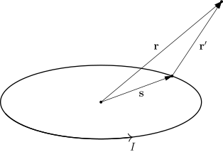
In our previous post, we created an electric dipole by taking two opposite charges infinitesimally close together. So today, in a similar spirit, we will create a magnetic dipole. We can model a magnetic dipole as a small loop of current $I$ with radius $a$. We can calculate the resulting magnetic field $\vb{B}$ by using the Biot-Savart law:
\[\vb{B} = \frac{\mu_0}{4\pi} \oint\limits_C \frac{I \dd{\vb{s}} \times \vb{r^\prime}}{\norm{\vb{r^\prime}}^3}\]Here, $\vb{s}$ represents the path of the current loop, and $\vb{r^\prime} = \vb{r} - \vb{s}$ represents the vector between the point $\vb{r}$ where the magnetic field $\vb{B}$ is calculated, and an infinitesimal segment $\dd{\vb{s}}$ of the current loop, located at position $\vb{s}$.
Since we are assuming a circular loop, we can write:
\[\begin{align} \vb{s} &= a \vu{e}_\rho^\prime \\ \dd{\vb{s}} &= a \vu{e}_\varphi^\prime \dd{\varphi^\prime} \\ \end{align}\]The prime here means that the vectors are functions of the variable of integration $\varphi^\prime$; unprimed quantities are not dependent upon $\varphi^\prime$, so they may be treated as constant with respect to the integral. Making these substitutions shown above, we obtain:
\[\begin{align} \vb{B} &= \frac{\mu_0 I}{4\pi} \oint\limits_C \frac{a \vu{e}_\varphi^\prime \dd{\varphi^\prime} \times (\vb{r} - a \vu{e}_\rho^\prime)} {\norm{\vb{r} - a \vu{e}_\rho^\prime}^3} \\ &= \frac{\mu_0 I}{4\pi} \int\limits_0^{2\pi} \frac{ a \vu{e}_\varphi^\prime \times \vb{r} - a^2 \vu{e}_\varphi^\prime \times \vu{e}_\rho^\prime }{ \qty( r^2 + a^2 - 2 a \vb{r} \cdot \vu{e}_\rho^\prime )^\frac{3}{2} } \dd{\varphi^\prime} \\ &= \frac{\mu_0 I}{4\pi} \int\limits_0^{2\pi} \frac{ a \vu{e}_\varphi^\prime \times \vb{r} + a^2 \vu{e}_z }{ \qty( r^2 + a^2 - 2 a \vb{r} \cdot \vu{e}_\rho^\prime )^\frac{3}{2} } \dd{\varphi^\prime} \\ \end{align}\]Without loss of generality, let $\vb{r} = r \vu{e}_z \cos(\theta) + r \vu{e}_x \sin(\theta)$, which gives:
\[\begin{align} \vb{B} &= \frac{\mu_0 I}{4\pi} \int\limits_0^{2\pi} \frac{ a \vu{e}_\varphi^\prime \times \qty[r \vu{e}_z \cos(\theta) + r \vu{e}_x \sin(\theta)] + a^2 \vu{e}_z }{ \qty( r^2 + a^2 - 2a \qty[r \vu{e}_z \cos(\theta) + r\vu{e}_x \sin(\theta)] \cdot \vu{e}_\rho^\prime )^\frac{3}{2} } \dd{\varphi^\prime} \\ &= \frac{\mu_0 I}{4\pi} \int\limits_0^{2\pi} \frac{ ar \, \vu{e}_\rho^\prime \cos(\theta) - ar \, \vu{e}_z \sin(\theta) \cos(\varphi^\prime) + a^2 \vu{e}_z }{ \qty[ r^2 + a^2 - 2ar \sin(\theta) \cos(\varphi^\prime) ]^\frac{3}{2} } \dd{\varphi^\prime} \end{align}\]But $\vu{e}_\rho^\prime = \vu{e}_x \cos(\varphi^\prime) + \vu{e}_y \sin(\varphi^\prime)$. Therefore, in an integral that involves some function of $\cos(\varphi^\prime)$, the $\sin(\varphi^\prime)$ term will yield zero. Hence:
\[\begin{align} \vb{B} &= \frac{\mu_0 I}{4\pi} \int\limits_0^{2\pi} \frac{ ar \, \vu{e}_x \cos(\theta)\cos(\varphi^\prime) - ar \, \vu{e}_z \sin(\theta) \cos(\varphi^\prime) + a^2 \vu{e}_z }{ \qty[ r^2 + a^2 - 2ar \sin(\theta) \cos(\varphi^\prime) ]^\frac{3}{2} } \dd{\varphi^\prime} \\ &= \frac{\mu_0 I}{4\pi} \int\limits_0^{2\pi} \frac{ ar \vu{e}_\theta \cos(\varphi^\prime) + a^2 \vu{e}_z }{ \qty[ r^2 + a^2 - 2ar \sin(\theta) \cos(\varphi^\prime) ]^\frac{3}{2} } \dd{\varphi^\prime} \end{align}\]So this is the expression we have for the magnetic field of a loop of current of macroscopic size. But in order to form a true magnetic dipole, we must let this loop of current have infinitesimal size. Therefore, we will calculate the Taylor expansion of $\vb{B}$ with respect to $a$. If we let $a \to 0$, then we see that $\vb{B} \to 0$, which means that the zeroth-order contribution to the Taylor series is zero. So we must compute the first derivative:
\[\begin{align} \pdv{\vb{B}}{a} &= \frac{\mu_0 I}{4\pi} \int\limits_0^{2\pi} \frac{ r \vu{e}_\theta \cos(\varphi^\prime) + 2a \vu{e}_z }{ \qty[ r^2 + a^2 - 2ar \sin(\theta) \cos(\varphi^\prime) ]^\frac{3}{2} } \dd{\varphi^\prime} \\ &+ \frac{\mu_0 I}{4\pi} \int\limits_0^{2\pi} \frac{ -3 \qty[ar \vu{e}_\theta \cos(\varphi^\prime) + a^2 \vu{e}_z] \qty[2a - 2r \sin(\theta) \cos(\varphi^\prime)] }{ 2\qty[ r^2 + a^2 - 2ar \sin(\theta) \cos(\varphi^\prime) ]^\frac{5}{2} } \dd{\varphi^\prime} \end{align}\]If we once again let $a \to 0$, then we see that a couple of terms survive, but they all involve $\cos(\varphi^\prime)$ by itself, which means that $\pdv{\vb{B}}{a} \to 0$ as well. So let us take the derivative one more time, but this time we will set $a\to 0$ immediately after differentiating, so as to not get a ridiculous number of terms:
\[\begin{align} \eval{\pdv[2]{\vb{B}}{a}}_{a = 0} &= \frac{\mu_0 I}{4\pi} \int\limits_0^{2\pi} \frac{2 \vu{e}_z}{\qty(r^2)^\frac{3}{2}} \dd{\varphi^\prime} \\ &+ \frac{\mu_0 I}{4\pi} \int\limits_0^{2\pi} \frac{-3\qty[r \vu{e}_\theta \cos(\varphi^\prime)] \qty[-2r \sin(\theta)\cos(\varphi^\prime)]} {2\qty(r^2)^\frac{5}{2}} \dd{\varphi^\prime}\\ &+ \frac{\mu_0 I}{4\pi} \int\limits_0^{2\pi} \frac{-3 [r\vu{e}_\theta \cos(\varphi^\prime)] [-2r\sin(\theta)\cos(\varphi^\prime)]} {2\qty(r^2)^\frac{5}{2}} \dd{\varphi^\prime} \end{align}\]We can combine all of these terms and simplify:
\[\begin{align} \eval{\pdv[2]{\vb{B}}{a}}_{a = 0} &= \frac{\mu_0 I}{4\pi} \qty[ 2\pi \qty(\frac{2 \vu{e}_z}{r^3}) + \int\limits_0^{2\pi} \frac{6\vb{r} \cos^2(\varphi^\prime) r \sin(\theta)} {r^5} \dd{\varphi^\prime} ] \\ &= \frac{\mu_0 I}{4\pi} \qty[ \frac{4\pi \vu{e}_z}{r^3} + \frac{6\pi r^2 \vu{e}_\theta \sin(\theta)} {r^5} ] \\ &= \frac{\mu_0 I}{r^3} \qty[ \vu{e}_z + \frac{3}{2}\vu{e}_\theta\sin(\theta) ] \\ \end{align}\]Hence, we see that the second-order contribution is the one that dominates the Taylor series of $\vb{B}$, since the zeroth and first order both contribute nothing. More explicitly,
\[\begin{align} \vb{B} &\approx \eval{\vb{B}}_{a=0} + \eval{\pdv{\vb{B}}{a}}_{a=0} a + \eval{\pdv[2]{\vb{B}}{a}}_{a=0} \frac{a^2}{2} \\ &= \eval{\pdv[2]{\vb{B}}{a}}_{a=0} \frac{a^2}{2} \\ &= \frac{\mu_0 I a^2}{2r^3} \qty[ \vu{e}_z + \frac{3}{2}\vu{e}_\theta\sin(\theta) ] \\ \end{align}\]This approximation becomes exact as we let the loop become smaller and smaller. We can rewrite this in terms of the area of the loop $\pi a^2$ to obtain:
\[\begin{align} \vb{B} &= \frac{\mu_0 I \pi a^2}{2\pi r^3} \qty[ \vu{e}_z + \frac{3}{2}\vu{e}_\theta\sin(\theta) ] \\ &= \frac{\mu_0 I \pi a^2}{4\pi r^3} \qty[ 2 \vu{e}_z + 3 \vu{e}_\theta\sin(\theta) ] \\ \end{align}\]And just like we did for electric dipoles, the correct limiting process involves taking $\pi a^2 \to 0$ and $I \to \infty$. Therefore, we may define the magnetic dipole moment as:
\[\vb{m} = I \pi a^2 \vu{e}_z\]Now, recall that we can express $\vu{e}_r$ and $\vu{e}_\theta$ as follows:
\[\begin{align} \vu{e}_r &= \vu{e}_z \cos(\theta) + \vu{e}_x \sin(\theta) \\ \vu{e}_\theta &= -\vu{e}_z\sin(\theta) + \vu{e}_x \cos(\theta) \\ \implies \vu{e}_\theta \sin(\theta) &= -\vu{e}_z \sin^2(\theta) + \vu{e}_x \cos(\theta)\sin(\theta) \\ &= -\vu{e}_z\sin^2(\theta) + \cos(\theta) \qty[\vu{e}_r - \vu{e}_z \cos(\theta)] \\ &= -\vu{e}_z + \vu{e}_r \cos(\theta) \\ \end{align}\]Hence, we can express $\vb{B}$ as follows:
\[\begin{align} \vb{B} &= \frac{\mu_0 m}{4\pi r^3} \qty[2 \vu{e}_z - 3\vu{e}_z + 3 \vu{e}_r \cos(\theta)] \\ &= \frac{\mu_0 m}{4\pi r^3} \qty[3 \vu{e}_r \cos(\theta) -\vu{e}_z] \\ &= \frac{\mu_0}{4\pi} \qty(\frac{3 m \cos(\theta)\vu{e}_r}{r^3} - \frac{m \vu{e}_z}{r^3}) \\ &= \frac{\mu_0}{4\pi} \qty(\frac{3 m (\vu{e}_z \cdot \vu{e}_r)\vu{e}_r}{r^3} - \frac{m \vu{e}_z}{r^3}) \\ &= \frac{\mu_0}{4\pi} \qty(\frac{3 (\vb{m} \cdot \vu{e}_r)\vu{e}_r}{r^3} - \frac{\vb{m}}{r^3}) \\ \implies \Aboxed{\vb{B} &= \frac{\mu_0}{4\pi} \qty(\frac{3 (\vb{m} \cdot \vb{r})\vb{r}}{r^5} - \frac{\vb{m}}{r^3})} \\ \end{align}\]So we see that a magnetic dipole has the exact same form as an electric dipole. How astonishing!