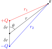
We can form an electric dipole by bringing two opposite charges $Q$ and $-Q$ together, each of them at a distance $\delta r$ from the origin. Let us examine their contribution to the electric potential at a point $\vb{r}$:
\[V = k \frac{Q}{r_1} - k \frac{Q}{r_2}\]We can then use the law of cosines to rewrite $r_1$ and $r_2$:
\[\begin{align} r_1^2 &= \delta r^2 + r^2 - 2 r \, \delta r \cos(\theta) \\ r_2^2 &= \delta r ^2 + r^2 - 2 r \, \delta r \cos(\pi - \theta) \\ \end{align}\]Therefore we see:
\[V = k Q \qty( \frac{1}{\sqrt{\delta r^2 + r^2 - 2 r \, \delta r \cos(\theta)}} - \frac{1}{\sqrt{\delta r^2 + r^2 + 2 r \, \delta r \cos(\theta)}} )\]Now, the idea is to bring these charges closer and closer together, meaning that $\delta r$ is infinitesimally small. Thus, we must use a Taylor approximation:
\[\frac{1}{\sqrt{x + \delta x}} \approx \frac{1}{\sqrt{x}} - \frac{\delta x}{2 x^\frac{3}{2}}\]When we apply this to our expression for the electric potential, we get:
\[\begin{align} V &\approx kQ \qty( \frac{1}{r} + \frac{-\delta r^2 + 2 r \, \delta r \cos(\theta)}{2 r^3} - \frac{1}{r} + \frac{\delta r^2 + 2 r \, \delta r \cos(\theta)}{2 r^3}) \\ &= kQ \, \frac{2 \delta r \cos(\theta)}{r^2} \\ \end{align}\]As we bring these charges closer and closer together, we must make $Q$ larger and larger; otherwise, the field will just tend to zero everywhere. This limiting process can be encapsulated by the electric dipole moment:
\[\vb{p} = 2 \delta r \, Q \vu{e}_z\]The electric potential can now be rewritten as:
\[\boxed{V = k \frac{\vb{p} \vdot \vb{r}}{r^3}}\]We can then take the gradient in spherical coordinates to obtain the electric field:
\[\begin{align} \vb{E} &= -\grad V \\ &= -k \qty(\vu{e}_r \partial_r + \frac{1}{r} \vu{e}_\theta \partial_\theta + \frac{1}{r \sin(\theta)} \vu{e}_\phi \partial_\phi) \qty(\frac{\vb{p} \vdot \vb{r}}{r^3}) \\ &= -k \qty(\vu{e}_r \partial_r + \frac{1}{r} \vu{e}_\theta \partial_\theta + \frac{1}{r \sin(\theta)} \vu{e}_\phi \partial_\phi) \qty(\frac{p \cos(\theta)}{r^2}) \\ &= -kp \qty(\vu{e}_r \partial_r \qty(\frac{\cos(\theta)}{r^2}) + \frac{1}{r} \vu{e}_\theta \partial_\theta \qty(\frac{\cos(\theta)}{r^2})) \\ &= -kp \qty( -2 \vu{e}_r \frac{\cos(\theta)}{r^3} - \vu{e}_\theta \frac{\sin(\theta)}{r^3} ) \end{align}\]Now, recall that we can express $\vu{e}_r$ and $\vu{e}_\theta$ as follows:
\[\begin{align} \vu{e}_r &= \vu{e}_z \cos(\theta) + \vu{e}_\rho \sin(\theta) \\ \vu{e}_\theta &= -\vu{e}_z \sin(\theta) + \vu{e}_\rho \cos(\theta) \\ \implies \vu{e}_z &= \vu{e}_r \cos(\theta) - \vu{e}_\theta \sin(\theta) \\ \end{align}\]We can then use this tool to rewrite the electric field:
\[\begin{align} \vb{E} &= -\frac{kp}{r^3} \qty[-2 \vu{e}_r \cos(\theta) - \vu{e}_\theta \sin(\theta) ] \\ &= -\frac{kp}{r^3} \qty[ -3 \vu{e}_r \cos(\theta) + \vu{e}_r \cos(\theta) - \vu{e}_\theta \sin(\theta) ] \\ &= -\frac{kp}{r^3} \qty[ -3 \vu{e}_r \cos(\theta) + \vu{e}_z ] \\ &= k \qty( \frac{3 (\vb{p} \vdot \vb{r})\vb{r}}{r^5} - \frac{\vb{p}}{r^3}) \\ \implies \Aboxed{\vb{E} &= \frac{1}{4\pi \varepsilon_0} \qty( \frac{3 (\vb{p} \vdot \vb{r})\vb{r}}{r^5} - \frac{\vb{p}}{r^3})} \\ \end{align}\]